Based on IoT, Big Data and Artificial Intelligence it’s possible to create a heat map of Volatile Organic Compounds, CO and particles matter pollution inside a chemical production plant. An agile system is needed to predict non-safe zones for i.e. pregnant and nursing women.

Monitoring air quality
Factory workers are exposed to several sources of work-related physical stress factors: loud and intense noise, heat and air pollution. Some of them, such as noise and heat can be easily measured and predicted. Other sources of pollution, like Volatile Organic Components, cannot be readily sensed and predicted. Nevertheless, they present a real danger for possible health problems.
The physical phenomenon of diffusion is theoretically well understood. Mathematically, it’s described by an equation known as Fick’s law:
 Fick’s law
Where:
- c is the concentration mol/m³ (or equivalent units)
- t is time [s]
- D is the diffusion coefficient [m²/s]
- x is the spatial dimension [m]
- s is the source term [mol/m³s]
The equation describes the transport of mass through diffusive means. It describes that there will be a solute flux along the concentration gradient. The solute will move from a position with high concentration to a neighboring position with lower concentration. The speed of this process is defined by the diffusion coefficient D. Using this equation, it’s possible to calculate the concentration in every position at any moment in time, assuming you know the starting condition, diffusion coefficient, source terms and boundary conditions. However, the latter is harder than it sounds.
In the context of modeling the air concentration of volatile chemical compounds in a chemical factory, the source terms are the chemical processes and production machines. Accurately measuring the emissions of each machine is possible, but it would require shutting down the complete factory and performing a high number of repetitive experiments and measurements for each machine operating under each possible setting. This would be a very costly procedure, both due to time consumption for the tests and the opportunity cost of stopping production.
Verhaert Masters in Innovation developed a tool and procedure to solve this problem based on real-time data from air quality monitoring called Smart Spot, provided by HOPU. The HOPU SmartSpot device, equipped with an ION Sensor MiniPID for volatile organic components, allows you to gather a large dataset of observational data. From this dataset, the unknown parameters can be inferred.
This ‘IoT – Big Data’ approach permits to gather data for the production of a large number of materials. The advantages?
- It combines monitoring with prediction: permanent temperature, noise and air pollution measurement allow to evaluate the current situation, independent from predictions.
- Data can be gathered during the normal operation of the factory.
- When the product portfolio changes, the new parameters can be learned by the system without further interference.
Using IoT & Big Data analysis methods to build a diffusion physics model
Discretization of Fick’s law
Fick’s law can be discretized. This allows to numerically solve the diffusion problem. This can be discretized on a rectangular m × n grid:
 Discretization of Fick’s law
- Where ℭ = {(i +/- 1, j),(i, j +/- 1)} is the set neighboring nodes to node (i,j);
- A is the diffusion surface between nodes k and (i,j);
- L is the distance between these nodes;
- g is a possible adjustment for the diffusion coefficient to take into account walls, doors and screens. Diffusion is not possible through a wall, the diffusion coefficient between nodes k and (i, j) at either side of a wall is there for 0.
This results in a matrix multiplication model. In this work, this model could be restricted to the steady-state case:
 Basic matrix multiplication model of the discretized Fick’s law (steady-state case)
![]() Steady-state case solution
Steady-state case solution
The result is c, a vector containing p = m.n-p concentrations that need to be determined. This is calculated based on the influence matrix G, a sparse p × p matrix containing the influence terms.
The influence of node i on node j is given by:
![]() Influence term of node i on node j
Influence term of node i on node j
This term is 0 for all pairs (i,j) that do not share a diffusion border. The diagonal elements (i,i) of the influence matrix contain the sum of all the terms of influence on node i.
![]() Sum of influence terms on node i
Sum of influence terms on node i
This influence matrix is combined with:
- s, the sparse vector containing the source terms
- The sink terms, listed in the vector f and their influence terms.
This is the result of a calculation with input values:
- Square map: 20 m × 20 m on a grid of 20 × 20 nodes
- 1 wall (g=0) in the middle, 15 m long
- 1 source of value 1 mol/m³s on position (2 m,5 m)
- 1 sink of value 0 mol/m³ on position (2 m,15 m)
- Diffusion coefficient D=0.1 s/m² (in a problem like this, the steady-state result is not influenced by the value of D).
The example below shows the steady-state IoT solution for the given (hypothetical) problem. The concentration value tag color has no meaning. It changes from black to white merely to optimize readability.
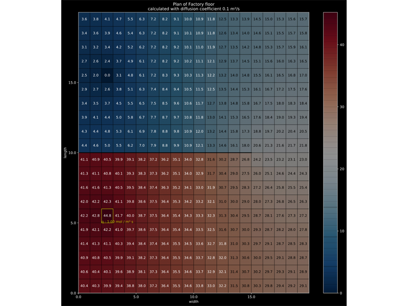 Result of the steady-state solution of Fick’s Law
Model calibration
Having an IoT tool to solve the diffusion problem with known source and sink terms is not a complete solution to our problem! The source and sink variables are unknown. In the context of modeling the air concentration of volatile chemical compounds in a chemical factory, these terms represent the amount of airborne chemicals produced by the chemical processes and production machines. These terms could be determined from individually testing each machine in controlled conditions.
For the IoT4Industry ‘Equality project’, we developed a proof of concept of a technique to infer these parameters from distributed observational measurements.
First, we need to be able to optimize a single diffusion map. Based on n measurements, the variables of a diffusion map can be estimated by minimizing the Mean Sample Error (MSE):
 Mean Squared Error loss term
The MSE expresses the difference between the calculated concentrations c(θ) and the measured concentrations c. By minimizing this term concerning the unknown parameter, these unknown parameters can be estimated. Usually, it’s not possible to find a solution for θ without residual error. In the illustration below, such a case is illustrated. Using the same geometry as in the previous example, we suppose to have two measurements, not that far from the source.
For the sake of the example, the source term is supposed to be a known parameter in this example. The unknown variable is the diffusion coefficient D. If a value of 2.7 mol/m3 is measured in two different points such as in this problem, there is no perfect analytical solution to this problem. The solution with minimized MSE is displayed on the right: the measured values of 2.7 mol/m3
are approximated with [2.6 ; 2.8]mol/m3 by estimating the diffusion coefficient to be 1.42 m²/s.
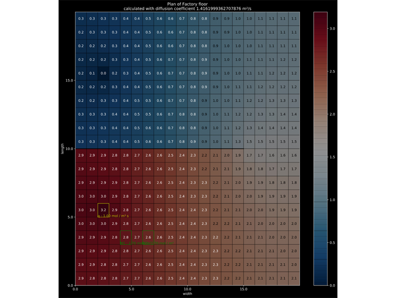 Best fit solution
Performing this optimization for a complete factory with a large product portfolio and complex production schedule is another challenge. A factory doesn’t produce the same product on the same production line every day. The challenge is to infer the contribution of each independent process from measurements of the combinations of these processes.
In practical settings, IoT sensor data isn’t always available for each sensing location at every moment. Sensors can break, but it’s also possible that sensors are rotated between measurement locations to increase covered location by the study while keeping the investment in individual sensors low. Consider the following simplified example on a (hypothetical) factory geometry as below:
 Table example case
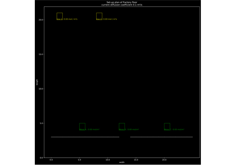 Hypothetical factory floor plan
Assume that in this factory, production line 1 and 2 are identical production units. When the same product is produced from the same material, these machines can be assumed to exhaust the same pollution levels.
Knowing the problem geometry, there are 3 unknown parameters in this problem:
- The production line exhaust during the production of recycled PVC;
- The line exhaust during the production of PE;
- The diffusion factor D.
This problem can be solved by minimizing the squared error for the complete factory problem consisting of the combination of S situations:
 Loss function over all situations
For the example discussed above, the result of this optimization is shown in the following figures:
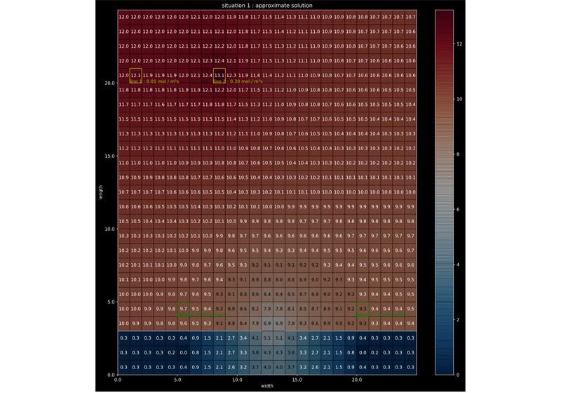 Approximation for situation 1
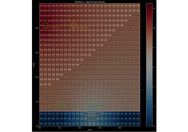 Approximation for situation 2
The developed model is applicable for a wide range of two-dimensional diffusion models, whether it is diffusion in air or liquids or other problems such as heat diffusion.
Application development
As production plant, Lisanplast has been the testing environment, a plastic extrusion company. Smart Spots were installed in different zones of the plant to collect the IoT data. These data are analyzed through a software platform based on Grafana, an Open Source technology that allows us to analyze all the data to obtain conclusions and export them to other tools and to create reports.
Verhaert’s AILab developed the app ‘Emission Predict Equality’ allowing the production manager of Lisanplast to estimate the zone-specific air contamination in his factory. So it’s possible to adapt the tasks and areas of work for a pregnant and nursing woman.
The final app is easy to use, the screen shows a simplified illustration of the Lisanplast floor plan where light green squares indicate the production line positions. Based on the production planning for this week, one can select the product, the type of plastic that will be processed for each of the 13 production lines, and the material mixer. The image below shows that on a typical day, the exposure limit of 50 µg/m³ PM10 is not expected to be breached. The contours indicate that around the extrusion heads of the production line one can expect that the PM10 level will reach 10% of this value. This zone is safe, but one might choose to avoid unnecessary presence in this zone.
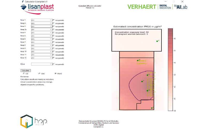 Screenshot of the developed application
Acknowledgment
The development of the calculator prototype and the approximation method was made possible thanks to the funding of IoT4Industry.
Watch the movie
Download the perspective
Looking for solutions to innovate?
Leave us your email and get in contact with Lieven Claeys, Business Development Manager Services ‘Digital Innovation’, to help you with your innovation process.